

Stabilized step, Mach displayed, a sweep sequence on the ailerons: the test room only watches one thing, by how much the damping of the second wing mode has decreased since the previous step. Not its value — its slope. An opening campaign never seeks flutter: it measures the speed at which the structure stops dissipating the energy it takes from the flow, and it stops before. What follows describes the excitation, modal identification, and the stop rule governing this progression.
Flutter is an energy transfer, not a strong vibration
An aircraft structure vibrates continuously without causing problems: turbulence excites it, its natural modes respond, structural and aerodynamic damping dissipate the received energy, the amplitude decreases. Flutter begins when this balance reverses. Two neighboring modes — classically the bending and torsion of a wing — couple through unsteady aerodynamic forces. If torsion gains a certain phase lead over bending, the unsteady lift works in the direction of motion each cycle: the flow gives energy to the structure instead of taking it.
Everything depends on a phase shift, which depends on geometry as much as speed. Three points govern the matter: the elastic axis, around which the section rotates; the center of gravity of the section; the aerodynamic focus, where the lift variation is applied. A center of gravity located aft of the elastic axis creates a torsional couple with each vertical acceleration — this is the inertial coupling, and the reason for the balance masses of the control surfaces.
Flutter happens when the wing starts getting energy from the airflow instead of losing it. This happens when the twisting motion of the wing gets slightly ahead of the bending motion, creating a dangerous feedback loop. The key is to detect this before it becomes dangerous.
On an Airbus A320, during flutter testing, engineers detected a critical phase shift at 0.85 Mach and 30,000 feet. The damping ratio for the second wing mode decreased from 0.05 to 0.025 over just 20 knots of speed increase, triggering an immediate stop of the test.
The practical consequence is brutal. Beyond the critical speed, the amplitude grows from one cycle to the next according to an exponential whose time constant is counted in fractions of a second for modes of a few hertz. There is no exploitable warning sign in piloting, nor any recovery maneuver: structural failure precedes reaction. Hence the method: do not approach until something is felt, but follow a quantity that, for its part, warns well in advance.
The same mechanism is found wherever an elongated structure bathes in a fast flow: control surfaces and flaps, tailplanes, masts and nacelles, and even the fan and compressor blades, whose flutter zones are mapped in regime and incidence like a speed domain.
What is measured in flight: modal damping, not a limit
The monitored quantity is the damping of each monitored mode, expressed as a fraction of critical damping or in the form of a structural damping coefficient. It is read on two inseparable plots, as a function of equivalent speed or dynamic pressure: the evolution of natural frequencies, and that of dampings. Flutter is not only announced by a damping that plummets; it is first announced by two frequencies that come together. This coalescence is the signature of the coupling being established.
An isolated mode whose damping slowly decreases is less worrying than two modes whose frequency difference closes step by step, even if their dampings remain comfortable. The first case may just be an unsteady aerodynamic effect without consequence; the second announces that the exchange mechanism is being set up.
That said, damping is an estimated quantity, not measured. It is obtained by fitting a model to a recorded response, and the estimation always comes with a dispersion. On a well-excited free response, with well-separated modes, the uncertainty remains low. On a turbulence signal, in a zone where three modes overlap, it can reach the order of magnitude of the variation one seeks to detect. A campaign is therefore judged as much by the quality of its excitations as by the sophistication of its processing.
Exciting the structure without jarring it
Making the structure speak requires injecting energy into the band of monitored modes — from a few hertz to a few tens of hertz on a transport aircraft — with a level sufficient to emerge from the noise and low enough to remain in the linear domain and far from fatigue limits. Five means coexist, and most campaigns combine several according to the domain zone.
| Moyen | Bande utile | Quality of the estimate | Contrainte |
|---|---|---|---|
| Manual pulse on a control surface | Broad but uncontrolled, energy decreasing with frequency | Adequate on the first modes, poor beyond | No installation, poor repeatability |
| Sweep injected by the flight control computer | Selected, limited by actuator bandwidth | Good, controlled signal-to-noise ratio | Injection law to develop, qualify and inhibit |
| Rotating-mass inertial exciter | Narrow and swept, energy increasing with the square of frequency | Very good on higher modes | Onboard mass, structural attachment, failure cases |
| Aerodynamic vane at the wing tip | Broad, energy increasing with dynamic pressure | Very good, including near the limit | Wing modification, drag, own qualification |
| Atmospheric turbulence alone | Broad, non-stationary, non-reproducible | Low: significant bias and scatter | None, but entirely dependent on the weather |
The choice is not only technical. An inertial exciter or a wing tip panel are modifications to the aircraft: to be installed, justified, monitored, and their failure in flight becomes a test case in itself. Flight controls, on the other hand, are already there — hence the appeal of sweeps injected by the computer, however limited by the bandwidth of the servocontrols and by the authority available at high speed, precisely where it would be most needed.
The pitfall of linear extrapolation. The damping curve often remains flat, sometimes slightly increasing, up to half a step from the limit, then collapses. Extending the last three points with a ruler reassures exactly where the plot ceases to be linear. Excitation by turbulence alone worsens the illusion: its dispersion, of the same order as the sought variation, turns a real drop into a cloud of points without a readable slope.
The step, unit of domain progression
The opening is conducted step by step. A step is a combination of altitude, Mach, and speed held long enough for the configuration to be stable, followed by a repeated excitation sequence, transmission of recordings by telemetry, and analysis rendered before the aircraft changes anything. The decisive point is the order: one does not advance until the previous step has been declared exploitable and compliant.
The increments tighten as progress is made. Far from the limit, they are counted in tens of knots or hundredths of Mach; as the domain edge is approached, they are halved, then again. This tightening is not symbolic: it follows the expected shape of the damping curve, which remains flat for a long time before dropping quickly.
The flight does not go up to the required margin. The domain that the aircraft will exploit is demonstrated in flight, up to the dive speed; the additional margin beyond, traditionally of the order of fifteen percent in equivalent speed, is established by aeroelastic calculation calibrated on the measurements. What is brought back from the flight is therefore not a speed, but a validated model, the only one capable of concluding where the aircraft will not go. Ground vibration tests play the same role upstream: they give the real frequencies and deformations of the cell, without which the model would start wrong from the first step.
The order of the steps depends on the transonic dip
The flutter speed does not evolve monotonically with Mach. It passes through a marked minimum in the transonic range, just below Mach 1, where the shock wave sets on the upper surface and moves with the angle of attack: the unsteady forces become very sensitive to motion, which degrades stability. The most constraining area of the domain is therefore not at the fastest corner of the envelope, but where the Mach is high without the dynamic pressure having decreased much.
Hence two ways of approaching, which are not equal. Increasing speed at constant altitude increases the dynamic pressure at moderate Mach: regular progression, readable trend, credible extrapolation from one step to the next. Descending at constant Mach increases it in a region where the limit itself collapses: two neighboring steps in speed can be very far apart in real margin. The transonic region receives for this reason its own increments, often built in Mach, and an excitation chosen to remain effective despite the aerodynamic shaking that pollutes the spectra.
The stop rule is written before the flight, not at the moment it is used
A stop criterion decided in the test room, under the pressure of a closing window, is worth nothing. Serious campaigns freeze before the first flight what triggers the stop, who makes the decision, and what the crew does in the following second: immediate reduction, exciter cutoff, heading and altitude for recovery. The stop authority belongs specifically to a position, usually the engineer in charge of aeroelasticity in the room, and it is exercised without discussion.
The criterion itself is almost never a single threshold on damping. It combines a floor — a percentage of critical damping below which one does not go — with a reading of trend and measurement quality.
| Observation | Interpretation | Decision |
|---|---|---|
| Stable damping, low scatter, well-separated frequencies | Margin intact, model in agreement | Next test point at the planned increment |
| Steady decrease, in line with the correlated prediction | Comportement compris | Next test point, reduced increment |
| Frequency gap between two modes closing | Coalescence under way | Minimum increment, closer monitoring of both modes |
| Decrease faster than predicted | Model wrong at this point of the envelope | Expansion stopped, reanalysis on the ground |
| Scatter above the criterion | Measurement not usable | Repeat the test point with stronger excitation |
| New mode, absent from the model | Configuration outside assumptions | Stop, return to the ground, model revision |
The right reflex: extrapolate a quantity that linearizes. Rather than damping alone, follow a margin indicator built from the frequencies and dampings of the two coupling modes: it varies much more regularly with dynamic pressure and supports an extrapolation from one step. And run two independent identification methods on the same recording: it is their discrepancy, more than the average value, that says whether the step is exploitable.
Configurations, masses and clearances: what shifts the limit
A flutter limit is demonstrated for a state, not for an aircraft. The filling of the wing tanks changes both the mass and its distribution: with full tanks, the bending frequencies decrease and the coupling shifts; with empty tanks, a mode that was not critical may become so. The deployment of slats, flaps, and landing gear, the carrying of external loads, the addition of antennas or fairings afterward all modify one of the three quantities that govern the phenomenon: mass, stiffness, damping.
Failure cases count as much as normal configurations. The loss of a control surface damper, the jamming of a servocontrol, the failure of an electrical flight control chain change the boundary conditions of the system, hence its stability. These cases are first treated by calculation; those that remain dimensioning are verified in flight, simulated failure, away from the domain edge.
The engine deserves special mention. Suspended from its pylon, it constitutes a significant mass whose natural modes — lateral sway, vertical sway, pylon torsion — couple with those of the wing, to the point that the stiffness of the attachments is part of the design levers. A re-engining, a change of nacelle, a pylon reinforcement reopen the aeroelastic file even when the wing is not touched.
The articulation clearance is the most banal and most dreaded parameter. An out-of-tolerance clearance on a control surface, a balance mass raised after repair without reweighing, an overcoat of paint on a moving surface: each of these deviations shifts a hypothesis of the demonstration. The system does not become unstable in the classical sense, it enters into sustained oscillation of bounded amplitude — without spectacular divergence, but with a consumption of fatigue life that nothing signals in the cockpit.
What the campaign leaves to those who operate the aircraft
There are few visible traces of a flutter campaign in a cockpit: a speed limit, sometimes a configuration restriction, and above all maintenance tasks whose purpose is not obvious as long as one has not seen their origin. Control of articulation clearance, verification of balance masses after repair of a control surface, paint thickness limit on certain moving surfaces, reweighing after intervention: these requirements come directly from the hypotheses held during the steps.
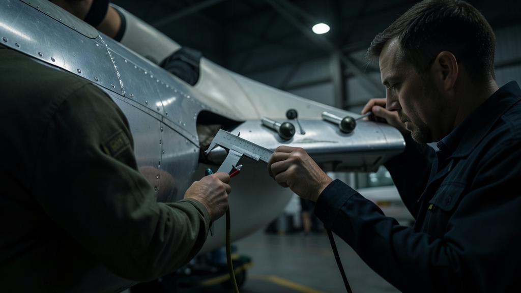
Link each clearance task to its hypothesis. Faced with a tolerance that seems disproportionate, look in the approved documentation for the moving assembly concerned and the associated balancing state: the value is not a mechanical comfort threshold, it is a condition of validity of the flutter-free demonstration. A repair that adds mass aft of a joint calls for a balance check, even if classified as minor otherwise.
Two gray areas remain. The first is that of limit cycle oscillations: bounded, non-divergent, they do not enter the strict definition of flutter, but they wear the structure and legitimately worry the crews; their treatment is handled on a case-by-case basis and often ends with an inspection instruction. The second is that of accumulated modifications — antennas, fairings, composite repairs — each of which is justified separately and whose combination has never been analyzed. It is a recurring subject of exchanges between practitioners after a trailing edge repair.
For those preparing a type qualification, a certifying personnel role, or a test office function, the useful thing is not to know how to calculate a critical speed: it is to know what questions to ask in the face of a modification. What added mass, where relative to which joint, what stiffness affected, what assumed clearance state. Check in your own documentation which configurations are covered and under what clearance and balancing conditions: it is there, and not in the chapter on speed limits, that the exploitable part of all this work is found — an angle that technical training courses rarely address head-on.
This article exposes mechanisms and does not replace anything: the applicable certification specifications, the acceptable means of compliance published by the authority, and the approved documentation of the operator prevail in all circumstances over what is described here.


Leave a Reply
You must be logged in to post a comment.