
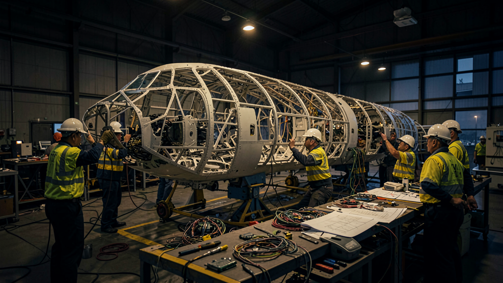
Every clean-sheet aircraft programme loses money on its first aeroplanes, and it is not because the early customers negotiated well — though they did. It is because the number of labour hours required to build serial number 5 is several times the number required to build serial number 500, and that decline follows a mechanism which is well described, measurable, and easy to destroy. Understanding the learning curve explains a great deal of industrial behaviour that otherwise looks irrational: why manufacturers resist design changes, why a rate increase can raise unit cost, and why a second assembly line does not simply double output.
An observation made in an aircraft factory in 1936
The idea comes from aviation, which is not a coincidence. In February 1936, T. P. Wright published « Factors Affecting the Cost of Airplanes » in the Journal of the Aeronautical Sciences, reporting something he had measured rather than theorised: as the cumulative number of airframes built increased, the average direct labour hours per airframe fell by a roughly constant percentage each time cumulative output doubled. For the airframe assembly work he was observing, that percentage was about twenty — an « 80 % curve » in the vocabulary that followed.
Three things about that statement matter and are routinely mangled. First, the driver is cumulative output, not calendar time. A factory that builds nothing learns nothing; a year of production at low rate teaches less than six months at high rate. Second, the reduction applies to a doubling, which means it slows dramatically in absolute terms: the step from unit 1 to unit 2 is the same percentage as the step from unit 500 to unit 1000, but there are 500 aeroplanes between the second pair. Third, it applies to touch labour — the hours a human spends on the aeroplane. Material content, purchased equipment and machine time follow their own, generally much flatter, curves.
The learning curve shows that as more aircraft are built, the time (and cost) to build each one drops. But this drop isn’t steady—it slows down as production grows. The first few planes take much longer to make than later ones, which is why early models are often sold at a loss.
The Airbus A350 program experienced steep learning curve effects. The first A350-900 took over 100,000 labor hours to build, while the 100th unit required only about 30,000 hours—less than a third of the initial effort. This dramatic reduction is why early deliveries are often unprofitable, while later ones become more cost-effective.
The arithmetic, and what it says about the first units
The unit form of the relationship is simple: H(n) = T1 × n^b, where H(n) is the hours needed for unit n, T1 is the hours for the first unit, and b = ln(r) / ln(2) with r the learning rate. An 80 % curve gives b ≈ −0.322; an 85 % curve gives b ≈ −0.234.
| Cumulative unit | 80 % curve | 85 % curve | 90 % curve | 95 % curve |
|---|---|---|---|---|
| 1 | 100 % | 100 % | 100 % | 100 % |
| 10 | 48 % | 58 % | 70 % | 84 % |
| 50 | 28 % | 40 % | 55 % | 75 % |
| 100 | 23 % | 34 % | 50 % | 71 % |
| 500 | 14 % | 23 % | 39 % | 63 % |
| 1000 | 11 % | 20 % | 35 % | 60 % |
The table answers the question in the title without further commentary. On an 80 % curve, unit 10 needs roughly three and a half times the labour of unit 500, and the first aeroplane off the line more than seven times as much. If the aeroplane is sold at a price that makes sense at unit 500 — and it must be, because that price was quoted years before either aeroplane existed — then the first dozens are built at a loss that was planned, budgeted and accepted before the programme was launched.
Note also what the right-hand columns show. A programme on a 95 % curve barely improves at all: after a thousand aeroplanes it is still spending 60 % of the first unit’s hours. The difference between a good curve and a poor one is not a matter of a few percentage points of margin; it decides whether a programme is viable.
Two models, one number, different meanings
A recurring source of confusion in cost discussions is that “an 80 % curve” describes two different models. Wright’s original formulation applies the decline to the cumulative average hours across all units built so far. The unit formulation — usually credited to Crawford, and standard in much US defence cost estimating — applies it to the hours of the individual unit. The same learning rate produces materially different unit hours in the two models.
| Cumulative unit | Unit hours, Crawford unit model | Cumulative average hours, Wright model | Approximate unit hours implied by the Wright model |
|---|---|---|---|
| 10 | 48 % of T1 | 48 % of T1 | about 32 % of T1 |
| 100 | 23 % of T1 | 23 % of T1 | about 15 % of T1 |
| 1000 | 11 % of T1 | 11 % of T1 | about 7 % of T1 |
The first two columns carry identical figures, and that is the whole difficulty: the same exponent is being applied to two different quantities. In the unit model it describes the hours of one aeroplane; in Wright’s model it describes the average across every aeroplane built so far, which means the individual unit at that point must be well below the average — the third column. A programme quoted at 80 % on the Wright convention is therefore forecasting fewer hours at unit 100 than the same rate quoted on the unit convention.
The practical consequence is that a learning rate quoted without its model is not information. Two estimates of the same programme, both honestly stated as 80 %, can differ by a third at unit 100. When comparing published figures — and manufacturers, suppliers and defence agencies do not all use the same convention — the model is the first thing to establish and the last thing anyone mentions.
What the hours on unit 1 are actually made of
It helps to be concrete about why the first aeroplane is so expensive in labour, because “inexperience” is only part of it and not the largest part.
- Immature work instructions. The written method exists but has never been executed; every ambiguity is resolved on the shop floor, by conversation, and each resolution costs time and generates a query.
- Tooling not yet proven. Jigs, fixtures and drilling templates are new. They fit approximately; the adjustments are found on the first articles.
- Travelled work. Parts arrive late or non-conforming, so work is performed out of station — in a position where access is poor, at a stage where it interferes with other work. Out-of-station work is expensive in a way that is roughly invisible in the plan and painfully visible in the hours.
- Rework and concessions. Early builds generate non-conformities at a rate that later builds do not, each requiring investigation, disposition and repair.
- Engineering change traffic. The definition is still moving. Each change means new instructions, new tools, and — critically — the operator starting again on that operation.
- Supply chain immaturity. Every supplier is on its own first units, with its own version of everything above.
- No takt stability. Without a stable rhythm, the line cannot be balanced, so labour sits idle in some stations and is overwhelmed in others.
Only one item on that list is about individual skill. The rest are properties of the process, and that is the key to everything that follows: the learning curve is a property of an organisation and its process, not of a serial number.
What actually makes the hours fall
Repetition alone produces only a fraction of the decline. The rest is deliberate work, and a programme that does not do it does not get the curve.
- Method engineering. Industrial engineers observe, re-sequence and re-write operations. This is the part of the decline that is engineered rather than accumulated, and a programme that does not staff it does not get the curve.
- Tooling maturity. Fixtures are corrected, then improved, then replaced with better ones designed with knowledge the first set did not have.
- Design-for-manufacture feedback. The shop floor tells engineering that a fastener is unreachable; the design changes once, early, and the operation loses hours permanently.
- Line balance and takt. Work is redistributed between stations so that no station is the permanent bottleneck.
- Supplier learning. The airframer’s curve is an aggregate of its suppliers’ curves. A supplier stuck at low rate holds the whole aggregate back.
- Automation, where it is justified. Automated drilling and fastening remove hours, but only become economic at a rate and a stability the early programme does not have — which is why automation usually arrives after the curve has already started falling.
The reflex that works. When a manufacturer announces a cost improvement, ask what changed in the process, not what changed in the hours. Hours are the output; process is the cause. A programme that reports falling hours and can name the method changes, tooling replacements and design revisions behind them has a real curve. One that reports falling hours after a rate increase and cannot name the cause is usually reporting a mix effect that will reverse. The mechanics of programme ramp-up are discussed regularly on the FL330 forums.
What stops the curve, or sends it backwards
The reason the learning curve is worth understanding is not that it works. It is that it stops working, predictably, for reasons that are usually decisions someone made.
| Mechanism | Effect on labour hours | Why |
|---|---|---|
| Stable design definition | Accelerates | An operation repeated identically is the only kind that can be learned |
| Engineering change traffic | Resets, operation by operation | New instructions and new tooling put the affected operation back near its own unit 1 |
| High customisation between units | Suppresses | If each aeroplane differs, the effective cumulative quantity for any given configuration is small |
| Rate increase with heavy hiring | Temporarily reverses | New operators dilute the experienced workforce; hours per unit rise before they fall |
| Supply disruption | Reverses | Forces out-of-sequence build and travelled work, the most expensive labour in the factory |
| Transfer to a second final assembly line | Partial restart | Only part of the learning transfers; the new site has its own workforce, tooling and suppliers |
| A long production gap | Reverses | Organisational forgetting is measurable; people leave and undocumented knowledge leaves with them |
| Loss of experienced staff | Reverses | Much of the learning lives in individuals, not in documents |
The trap. The most expensive misreading in the industry is treating the learning curve as automatic — as something a programme is entitled to because it has built a certain number of units. It is not a law of nature; it is the summed result of a stable definition, a stable workforce and continuous method work. Change any of the three and the hours stop falling regardless of what the serial numbers say. Programmes that budgeted the curve as an assumption rather than earning it as a result have produced some of the largest write-downs in commercial aerospace.
Learning is not rate, and rate is not learning
These two are constantly conflated in public discussion and they are separate quantities. The learning curve describes hours per aeroplane. Rate describes aeroplanes per month. A factory can be excellent at one and incapable of the other.
Rate is limited by physical capacity — stations, jigs, floor space, the takt time the tooling permits — by workforce size, and above all by the slowest supplier. Learning is limited by the stability of the process. Increasing rate usually damages learning in the short term, because the hiring required to do it dilutes the experienced workforce and the extra demand strains suppliers who are themselves early on their own curves. The commercial pressure to ramp up is therefore in direct tension with the industrial requirement to let the curve run — which is the entire drama of every ramp-up in the industry’s history, restated with new aircraft types.
What the curve does to the money
Recurring labour is only one component of unit cost, but its trajectory dominates programme economics in the early years, and accounting treatment determines how visible that is.
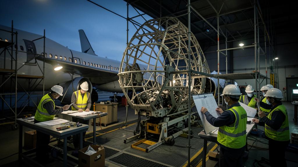
Under US GAAP, programme accounting allows a manufacturer to spread costs across a defined accounting quantity of aircraft rather than recognising them unit by unit — meaning the loss on early units is deferred and recovered against later, cheaper ones. The mechanism is legitimate and rests entirely on the assumption that the curve arrives as forecast. When it does not, the deferred balance grows: the 787 programme’s deferred production cost ran into the tens of billions of dollars at its peak — a curve that did not arrive on schedule, expressed in a balance-sheet line. IFRS does not permit that treatment, so European manufacturers recognise cost against each unit as it is delivered, and the early loss appears immediately rather than being carried forward.
Two further effects compound the early loss. Launch customers buy at discounts negotiated when the programme needed orders more than margin, so the cheapest aeroplanes to buy are the most expensive to build. And non-recurring cost — development, certification, tooling — sits on top of all of it, needing to be recovered from a delivery stream that has not yet begun to be profitable. Cumulative cash breakeven on a clean-sheet commercial programme is typically several hundred aircraft away, sometimes far more, and some programmes never reach it at all.
This is also why derivatives are so attractive. A re-engined or stretched version inherits a mature airframe process, a trained workforce and proven tooling. It does not restart at unit 1; it joins an existing curve well down its slope. The commercial logic that keeps decades-old fuselage cross-sections in production is not conservatism. It is the arithmetic in the first table, read from the right-hand end.


Leave a Reply
You must be logged in to post a comment.